Examples#
Example 1: Single-bin LOSVD inference#
The simplest use case is a single spatial bin containing \(N\) stars with individual velocity measurements and uncertainties.
import numpy as np
from veldist import KinematicSolver

rng = np.random.default_rng(42)

# Intrinsic LOSVD: Gaussian with V = 0, σ = 20 km/s
n_stars = 200
v_int = rng.normal(0.0, 20.0, n_stars)

# Per-star measurement errors, drawn from a realistic range
errors = rng.uniform(5.0, 15.0, n_stars)
v_obs = v_int + rng.normal(0.0, errors)

# Set up the velocity grid and run inference
solver = KinematicSolver()
solver.setup_grid(center=0.0, width=200.0, n_bins=50)
solver.add_data(vel=v_obs, err=errors)
solver.run(num_warmup=500, num_samples=1000, gpu=False)

solver.plot_result()
The grid should comfortably enclose the data (\(\pm 3\sigma_\mathrm{obs}\) is a reasonable starting point) and the bin width \(\Delta v = \mathrm{width} / n\_\mathrm{bins}\) should be comparable to the typical measurement uncertainty. Making \(\Delta v\) much smaller than \(\varepsilon_\mathrm{typ}\) adds bins that the data cannot resolve; the prior will fill them in, but the posterior will be correspondingly wider.
Recovering a non-Gaussian LOSVD#
The same setup applies for non-Gaussian distributions. Here we use a double-peaked LOSVD, as might arise from a counter-rotating component or a contaminating background population:
# Two-component LOSVD: prograde and retrograde populations
n1, n2 = 150, 100
v_int = np.concatenate([
    rng.normal(-30.0, 12.0, n1),   # prograde component
    rng.normal(+50.0, 15.0, n2),   # secondary component
])
errors = rng.uniform(8.0, 18.0, n1 + n2)
v_obs = v_int + rng.normal(0.0, errors)

solver = KinematicSolver()
solver.setup_grid(center=10.0, width=250.0, n_bins=60)
solver.add_data(vel=v_obs, err=errors)
solver.run(num_warmup=500, num_samples=1000, gpu=False)

solver.plot_result()
A Gauss-Hermite fit would assign anomalously large \(h_3\) or \(h_4\) values to
such a distribution; the histogram representation captures both peaks directly.
The bimodality_score returned by compute_summary will be \(\geq 2\) for
bins where this structure is genuinely supported by the data.
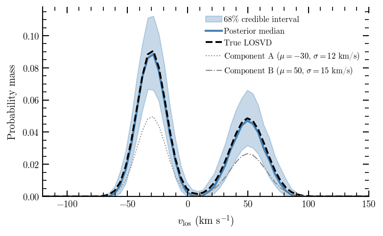
Posterior median (solid) with 68% credible interval (shaded) for the two-component example above. The dashed line is the true intrinsic distribution. Bins where the uncertainty interval is wide are those poorly constrained by the data; the prior keeps them smooth rather than noisy.
Example 2: Batch inference and Dynamite output#
For IFU-style data where stellar velocities have been Voronoi-binned, use
fit_all_bins to run inference across all bins and write_dynamite_kinematics
to produce the three files expected by Dynamite’s histLOSVD kinematics
handler.
Preparing the input#
fit_all_bins expects a list of dicts, one per Voronoi bin:
# bin_data_list[i] = {'vel': array, 'err': array} for bin i
# Bins with fewer than min_stars stars are skipped and returned as None.
bin_data_list = [
    {'vel': bin_velocities[i], 'err': bin_errors[i]}
    for i in range(n_bins)
]
Running the batch pipeline#
from veldist import fit_all_bins, write_dynamite_kinematics

solvers = fit_all_bins(
    bin_data_list,
    grid_kwargs={"center": 0.0, "width": 600.0, "n_bins": 60},
    run_kwargs={"num_warmup": 500, "num_samples": 1000, "gpu": False, "seed": 5567},
    min_stars=10,
)
fit_all_bins uses seed + bin_index internally so that the chains for
different bins are independent. Bins with fewer than min_stars stars are
returned as None and masked automatically in the output files.
Writing Dynamite input files#
# voronoi_bin_metadata describes the spatial layout of the IFU mosaic.
# See write_dynamite_kinematics docstring for the full required structure.

write_dynamite_kinematics(
    solvers=solvers,
    output_dir="dynamite_input",
    voronoi_bin_metadata=voronoi_bin_metadata,
    bin_flux_mode="nstars",   # use N_stars as the bin flux proxy
)
This writes three files to dynamite_input/:
bayes_losvd_kins.ecsv— one row per solved bin, with interleavedlosvd_j/dlosvd_jcolumns matching the BayesLOSVD ECSV format. Thedlosvd_jvalues are half-widths of the 68% credible interval, consistent with the convention used by Falcón-Barroso & Martig (2021).aperture.dat— pixel grid geometry for Dynamite.bins.dat— pixel-to-bin mapping; skipped bins are written as 0.
The bin_flux column receives solver.n_stars for each bin when
bin_flux_mode='nstars'. This is the natural discrete-data analogue of IFU
surface brightness. Note that bin_flux is used only for flux-weighted
systemic velocity centering (center_v_systemic) in Dynamite and does not
enter the NNLS chi-squared.
Optional post-processing#
clip_uncertainties() is called automatically inside fit_all_bins and
enforces a floor on dlosvd values to prevent zero-uncertainty entries in
the ECSV, which would corrupt Dynamite’s matrix inversion.
truncate_losvd() is available as an optional step for bins where significant
probability mass has accumulated in edge bins that are not supported by the
data (typically a sign that the grid is too wide or that the bin has very few
stars). It is not applied by default.
# Inspect a specific bin for tail contamination before deciding
solver = solvers[i]
solver.plot_result()

# Apply truncation only if clearly warranted
solver.truncate_losvd(n_sigma=3.0)
Example 3: Kinematic summary maps#
Once the batch pipeline has run, compute_summary_maps extracts
spatially-mappable scalar summaries from the posterior samples, analogous to
the \(V\), \(\sigma\), \(h_3\), \(h_4\) maps produced by Gauss-Hermite fitting.
from veldist.analysis import compute_summary_maps

maps = compute_summary_maps(solvers)
maps is a dict with one entry per metric; each entry contains 'median'
and 'uncertainty' arrays of length n_bins, with NaN for skipped bins.
Plotting kinematic maps#
import matplotlib.pyplot as plt
import matplotlib.colors as mcolors

xbin = np.array([meta['xbin'] for meta in voronoi_bin_metadata['bins']])
ybin = np.array([meta['ybin'] for meta in voronoi_bin_metadata['bins']])

metrics = [
    ('v_mean',    'Mean velocity (km s$^{-1}$)',     'RdBu_r'),
    ('sigma',     'Dispersion (km s$^{-1}$)',         'viridis'),
    ('skewness',  'Skewness $\\gamma_1$',             'PuOr'),
    ('kurtosis',  'Excess kurtosis $\\kappa$',        'PuOr'),
]

fig, axes = plt.subplots(1, 4, figsize=(16, 4))
for ax, (key, label, cmap) in zip(axes, metrics):
    vals = maps[key]['median']
    vmax = np.nanpercentile(np.abs(vals), 95)
    norm = mcolors.TwoSlopeNorm(vcenter=0, vmin=-vmax, vmax=vmax) \
           if cmap == 'RdBu_r' or cmap == 'PuOr' else None
    sc = ax.scatter(xbin, ybin, c=vals, cmap=cmap, norm=norm, s=30)
    plt.colorbar(sc, ax=ax, label=label)
    ax.set_aspect('equal')
    ax.set_xlabel('x (arcsec)')
    ax.set_ylabel('y (arcsec)')
fig.tight_layout()
Relationship to Gauss-Hermite moments#
The moment-based metrics from compute_summary are related to the
Gauss-Hermite coefficients by the following approximate conversions, valid
for \(|h_3|, |h_4| \lesssim 0.2\):
These allow direct cross-comparison with GH-based Dynamite models and with published kinematic maps from IFU surveys. Note the sign: \(\gamma_1 > 0\) (a trailing low-velocity tail) corresponds to \(h_3 < 0\), which is the expected pattern on the receding side of a rotating system.
The tail_weight metric and the bimodality_score have no GH analogues
and are diagnostic of features that GH fitting cannot represent — heavy tails
in the radially-anisotropic regime and genuinely bimodal LOSVDs from
kinematically distinct populations.

Example kinematic maps (\(V\), \(\sigma\), \(\gamma_1\), \(\kappa\)) from a synthetic globular cluster with a rotating core. The \(V\) and \(\sigma\) maps recover the known input rotation and dispersion profile; the \(\gamma_1\) map shows the expected antisymmetric pattern associated with rotation.