Methodology#
Overview#
veldist recovers the intrinsic line-of-sight velocity distribution (LOSVD)
from a discrete set of stellar velocities, each measured with its own
uncertainty. The approach is non-parametric: rather than assuming the LOSVD
follows a Gaussian or Gauss-Hermite expansion, we solve for the probability
mass in each bin of a fixed velocity histogram. Regularisation is provided
by a Gaussian random walk prior, whose smoothing scale is treated as a free
hyperparameter and marginalised over during inference. Measurement errors
enter the likelihood exactly, with no assumptions about their distribution
across stars.
The method is closest in spirit to the penalised-likelihood approach of Merritt (1997) and Saha & Williams (1994), but replaces the manual smoothing penalty with a marginalised Bayesian prior and uses MCMC sampling rather than optimisation.
The Model#
Histogram representation#
We represent the intrinsic LOSVD as a vector of probability masses \(\mathbf{w} \in \mathbb{R}^K\) on a fixed velocity grid with \(K\) bins, where \(\sum_j w_j = 1\). The grid is defined by a central velocity, total width, and number of bins. The bin width \(\Delta v\) is chosen to be comparable to the typical measurement uncertainty, so that the data can resolve individual bins.
Smoothing prior#
A flat histogram is not a useful prior for stellar kinematics: real LOSVDs are smooth. We impose this by generating the histogram weights through a latent Gaussian random walk. The latent variable \(u_i\) for bin \(i\) is drawn from a normal distribution centred on the previous bin value:
The weight vector \(\mathbf{w}\) is then obtained by applying the softmax transformation to \(\mathbf{u}\), which ensures positivity and unit normalisation.
The smoothing scale \(\sigma_\mathrm{smooth}\) controls the typical step size between adjacent bins. A small value forces the inferred LOSVD to vary slowly; a large value allows sharp features. Crucially, \(\sigma_\mathrm{smooth}\) is not fixed by the user — it is a free hyperparameter with a weakly informative prior, and its posterior is marginalised during sampling. The sampler therefore adapts the smoothness to the signal-to-noise of the data automatically: a bin with many stars will support more structure than one with few.
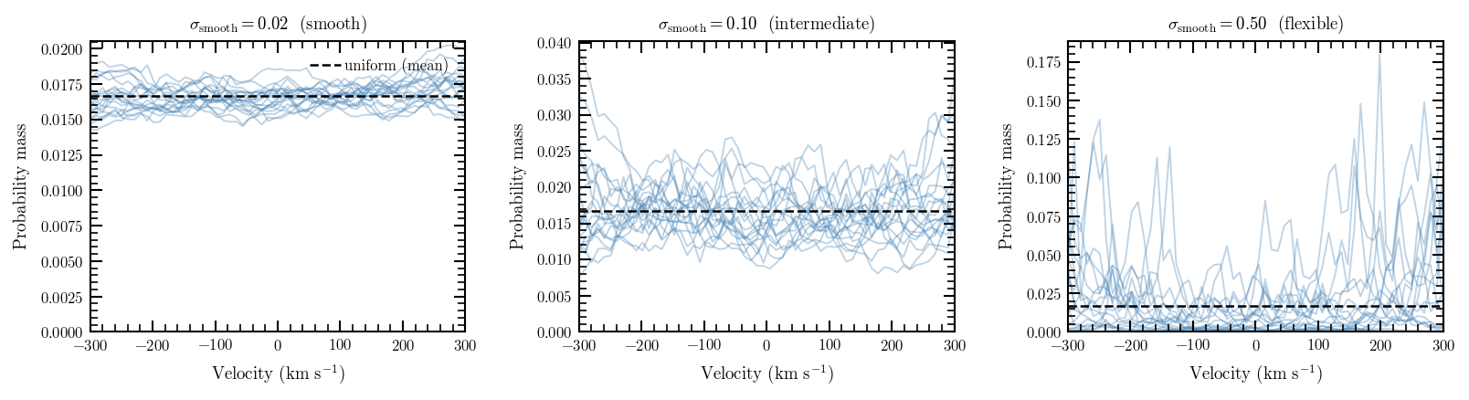
Prior realisations at \(\sigma_\mathrm{smooth} = 0.02\) (left), \(0.1\) (centre), and \(0.5\) (right). Lighter values of \(\sigma_\mathrm{smooth}\) enforce smoother LOSVDs; larger values allow the prior to explore more structured shapes. In practice the sampler marginalises over this parameter.
The Likelihood: Design Matrix#
The deconvolution problem#
The central difficulty is that every star has a different measurement uncertainty \(\varepsilon_i\). The observed velocity \(y_i\) of star \(i\) is drawn from a distribution that is the convolution of the intrinsic LOSVD with the star’s measurement error kernel:
where \(c_j\) is the centre of bin \(j\). Evaluating this naïvely for all \(N\) stars at every MCMC step is an \(O(N K)\) operation that involves \(N K\) exponential evaluations — expensive for large samples.
Pre-computing the design matrix#
We avoid this by pre-computing the \(N \times K\) design matrix \(\mathbf{M}\) before inference begins. Entry \(M_{ij}\) is the probability that star \(i\) would be observed in its measured position, given that it originates from intrinsic bin \(j\). Since \(y_i \sim \mathcal{N}(c_j, \varepsilon_i^2)\), this is the integral of the Gaussian error kernel over the bin extent \([c_j - \Delta v/2,\, c_j + \Delta v/2]\):
where \(\Phi\) is the standard normal CDF. This is computed once from the observed velocities and errors, and held fixed throughout inference.
Each row of \(\mathbf{M}\) corresponds to one star and has the shape of a Gaussian centred at \(y_i\) with width \(\varepsilon_i\), sampled at the grid bins. Stars with large errors have broad, flat rows; stars with small errors have narrow, peaked rows concentrated in one or two bins.
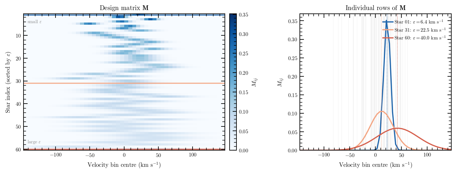
Left: the full \(\mathbf{M}\) matrix for a small example dataset, with stars ordered by measurement error. Right: three individual rows, showing how the per-star error kernel is integrated over the velocity bins. Stars with large \(\varepsilon_i\) (top row) contribute broad constraints; stars with small \(\varepsilon_i\) (bottom row) constrain a narrow range of bins.
Likelihood evaluation#
Once \(\mathbf{M}\) is available, the likelihood of the observed data given the weight vector \(\mathbf{w}\) is:
The product \(\mathbf{M}\mathbf{w}\) is a single matrix–vector multiplication: an \(O(NK)\) operation with no exponential evaluations inside the MCMC loop. This is the key computational advantage of the design-matrix approach: the expensive integrals are computed once at setup time, and inference itself requires only linear algebra.
Inference#
Posterior sampling is performed with the No-U-Turn Sampler (NUTS; Hoffman & Gelman 2014) as implemented in NumPyro (Phan et al. 2019). NUTS is a gradient-based Hamiltonian Monte Carlo variant that adapts its step size and trajectory length automatically, making it well suited to the high-dimensional posteriors that arise for fine velocity grids.
The sampler simultaneously infers \(\mathbf{u}\) (the latent random walk,
from which \(\mathbf{w}\) is derived) and \(\sigma_\mathrm{smooth}\). The
posterior over \(\mathbf{w}\) therefore marginalises over the smoothing scale,
propagating its uncertainty into all derived quantities. Users can run on
GPU by passing gpu=True to KinematicSolver.run(), which can reduce wall
time by an order of magnitude for large batches.
The default chain settings (500 warmup, 1000 samples) are sufficient for typical globular-cluster or dwarf galaxy bins with \(\gtrsim 30\) stars. For bins with \(N_\star \lesssim 20\) or for grids finer than \(\Delta v \sim \varepsilon_\mathrm{typ}\), the posterior will be prior-dominated; this is expected behaviour and the uncertainty intervals will reflect it.
Relationship to Prior Work#
Merritt (1997); Saha & Williams (1994)#
Both papers introduced the design-matrix formulation for LOSVD recovery from
discrete stellar velocities, with regularisation through a roughness penalty
applied to \(\mathbf{w}\) (penalised likelihood). The penalty scale \(\lambda\)
was chosen by the user or estimated from the data. veldist replaces the
fixed penalty with a Gaussian random walk prior whose scale is marginalised
during sampling; this avoids manual tuning and provides formal uncertainty
estimates on the smoothing scale itself.
Falcón-Barroso & Martig (2021) — BayesLOSVD#
BayesLOSVD introduced a Bayesian, non-parametric LOSVD extraction framework
for IFU spectra, using MCMC regularisation and a similar random walk prior.
The key difference is the data model: BayesLOSVD operates on integrated-light
spectra and requires a template stellar library and a deconvolution step with
the instrumental line-spread function. veldist targets discrete stellar
velocities, where the data are individual measurements with per-star error
bars — no template is needed. The design-matrix likelihood is specific to
this regime and cannot be used for spectral fitting.
veldist uses the BayesLOSVD ECSV file format for Dynamite input, which
allows the two codes to be used in sequence: veldist extracts LOSVDs from
resolved stellar data, which are then passed to Dynamite’s histLOSVD
kinematics handler.
Bovy, Hogg & Roweis (2011) — Extreme Deconvolution#
Extreme Deconvolution (XD) also handles heteroscedastic per-object errors,
but models the intrinsic distribution as a mixture of Gaussians rather than
a non-parametric histogram. The mixture representation is efficient when the
distribution is approximately Gaussian or a small sum of Gaussians, but
cannot represent flat-topped, asymmetric, or multimodal LOSVDs without a
large number of components. veldist makes no shape assumption; the prior
simply favours smooth solutions over rough ones.